Sagittal MSM
A faster approach to multi-scalar multiplication (MSM) of elliptic-curve points, one of the most expensive steps in zero-knowledge proving. This page explains it from the ground up, with step-by-step animations.
I invented the mathematical approach in 2022, built Python operation models and a C++ reference, then directed and reviewed the CPU and GPU implementations at Sindri Labs with colleagues and a Draper Labs contractor. The benchmark results below were a crucial part of the technical case behind Sindri's $5M seed round, led by CoinFund.
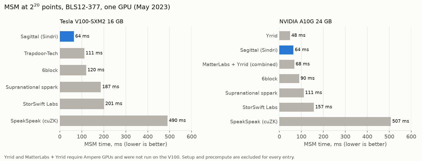
On BLS12-377 at 220 points, with the proving key precomputed once and reused across proofs, Sagittal ran an MSM in 64 ms: 1.7× faster than every ZPrize 2022 GPU entry that runs on a V100, and faster than all entries but one (Yrrid, 48 ms) on an A10G.
1. MSM and elliptic-curve arithmetic
A zero-knowledge proof lets a prover convince a verifier that a computation was done correctly without revealing its inputs. Most proof systems in use (Groth16, PLONK, and anything built on KZG polynomial commitments) commit to large polynomials, and committing to a polynomial with n coefficients is one MSM of n points. That is why MSMs dominate proving time.
A dot product
A dot product multiplies two lists pairwise and adds up the results. A multi-scalar multiplication (MSM) has the same shape, except the second list holds elliptic-curve points instead of numbers:
The scalars ki are ordinary integers, about 253 bits long. The points Pi are pairs (x, y) of 377-bit numbers. In a zero-knowledge prover the points are fixed (they come from the proving key and are the same for every proof of a circuit) and the scalars change every proof. Anything computed from the points alone can be computed once and reused.
Why 253 bits and 377 bits? There are two different primes. Coordinates are numbers modulo p, a 377-bit prime: the field. The points themselves form a group with r elements, where r is a 253-bit prime, so adding any point to itself r times gives the identity point O (defined below) and only k mod r matters. Scalars are numbers modulo r; coordinates are numbers modulo p.
Adding two points
The curves here have the equation y² = x³ + b (b = 1 for BLS12-377). Over the real numbers, adding two points has a picture: draw the line through P and Q, find where it meets the curve again, and reflect across the x-axis. Real curves use the same formulas with every number taken modulo a 377-bit prime. There is also an identity point O (the "point at infinity"): P + O = P, and P + (−P) = O, where −P = (x, −y).
λ  = (y₂ − y₁) / (x₂ − x₁)      for doubling: λ = 3x₁² / (2y₁)
x₃ = λ² − x₁ − x₂
y₃ = λ(x₁ − x₃) − y₁
Modulo p, dividing means multiplying by an inverse, which costs hundreds of multiplications. So implementations carry a running denominator in extra coordinates and divide once at the end. A point stored as plain (x, y) is affine. Jacobian coordinates store (X, Y, Z) with x = X/Z² and y = Y/Z³; XYZZ coordinates store (X, Y, ZZ, ZZZ) with x = X/ZZ and y = Y/ZZZ, the form the fastest GPU MSMs use. One addition then costs about 10–16 field multiplications: 10 for a mixed add (a running sum + a stored affine point), 14 for a full add (two running sums) and 9 for a doubling, in XYZZ.
Sagittal's GPU kernel kept its running sums (the buckets of sections 3 and 4) in Jacobian coordinates and its precomputed table entries affine, so each lookup is a mixed add. These are the exact formulas it ran, with every value in Montgomery form (see section 2): each product or square is one Montgomery multiplication, and additions and small multiples are ordinary modular additions.
Mixed add: (X1, Y1, Z1) + (x2, y2)        7 multiplications + 4 squarings
  Z1Z1 = Z1²
  U2   = x2 · Z1Z1                        x2 scaled to the bucket's denominator
  S2   = y2 · Z1 · Z1Z1                   y2 scaled likewise
  H    = U2 − X1                          x-difference (λ's denominator)
  HH   = H²,   I = 4·HH,   J = H · I
  r    = 2 · (S2 − Y1)                    y-difference (λ's numerator)
  V    = X1 · I
  X3   = r² − J − 2·V
  Y3   = r · (V − X3) − 2 · Y1 · J
  Z3   = (Z1 + H)² − Z1Z1 − HH            = 2·Z1·H, the new denominator

Double: 2·(X1, Y1, Z1)                    2 multiplications + 5 squarings
  A = X1²,   B = Y1²,   C = B²
  D = 2 · ((X1 + B)² − A − C)             = 4·X1·B
  E = 3 · A,   F = E²                     3x² from the tangent slope 3x²/(2y)
  X3 = F − 2·D
  Y3 = E · (D − X3) − 8·C
  Z3 = 2 · Y1 · Z1
From the
Explicit-Formulas
Database, where they are madd-2007-bl (mixed addition, Bernstein and Lange,
2007) and dbl-2009-l (doubling, Lange, 2009).
There is no multiply
A curve has only addition. "k·P" means adding P to itself k times. There is no way to multiply a point by a number directly, or to multiply two points, and recovering k from k·P (the discrete logarithm) is believed infeasible. That is what makes these curves useful for cryptography. Instead, double-and-add reads k's bits from the top: double at every bit, add P at every 1.
A 253-bit scalar takes about 252 doublings and 126 additions: 376 curve operations per point, measured. A naive MSM does that for every point, about 400 million curve operations at 220 points.
2. Big numbers and GPUs
Numbers bigger than a machine word
A machine word is the size of number a processor handles in one instruction: 64 bits on a CPU and 32 bits for a GPU's integer units. A 377-bit number is stored as 12 words of 32 bits, and multiplying two of them works like long multiplication on paper, one word pair at a time:
The product then has to be reduced mod p back to 12 words. Done directly, that is a long division, slower than the multiplication itself. Montgomery form avoids it: store each value a as a·R mod p, with R = 2384. Multiplying two stored values gives abR², and getting back to abR means dividing by R, which for a power of 2 just drops the low words. Values are converted in once at the start and out once at the end. Sindri's GPU code kept everything in Montgomery form.
The standard way to compute one Montgomery multiplication, CIOS (Coarsely Integrated Operand Scanning; Koç, Acar and Kaliski, 1996), interleaves multiplying and reducing word by word. It takes 2s² + s word multiply-adds for s words: 300 per field multiplication, and about 3,000 per curve addition.
GPU memory and threads
A GPU program is called a kernel (CUDA guide). It runs as thousands of threads, organized two ways: blocks of up to 1,024 threads that share a block of fast on-chip memory and can wait for each other, and warps of 32 threads that execute one instruction together. Threads in a warp that need to do different things wait for each other. Memory comes in tiers:
Why data-dependent work is costly
In Pippenger's bucket method the bucket a point goes to depends on its scalar, so many threads can target the same bucket at once. A bucket update is a curve addition (about 3,000 multiply-adds), not one instruction, so the GPU's atomic add (a hardware instruction that lets many threads add to the same number safely) can't do it: threads must take turns, or the points must be sorted by bucket first. Draw new scalars and compare one warp of 32 threads:
Fast implementations avoid the collisions by sorting points by bucket and balancing bucket sizes, and the ZPrize winners do that very well. But it is extra work every proof. An algorithm whose work is fixed in advance doesn't pay it.
3. Pippenger's bucket method
Every fast MSM builds on this (Bernstein on Pippenger). With n points, write each scalar in base 2c: c-bit digits called windows. In each window every point goes into the bucket for its digit. Then a running sum from the top bucket down computes Σ d·bucket[d] with about two additions per bucket, and windows are combined by doubling c times between them. Step through 8 scalars with c = 4:
The best window grows with n: c = 17 at 220 points, which means 15 windows × 65,536 buckets ≈ 983,000 buckets, filled by the data. (65,536 is 216, not 217: signed digits halve the buckets.) The ZPrize 2022 winners (Yrrid and MatterLabs) also precompute shifted copies of every point so all windows fold into a few bucket sets.
4. Sagittal MSM
Pippenger cuts the scalar bit matrix into strips c bits wide and n rows tall. Sagittal cuts it into blocks 1 bit wide and g rows tall. A block's g bits select one subset sum of its batch's points. That sum depends only on the points, so every subset sum is precomputed once per proving key.
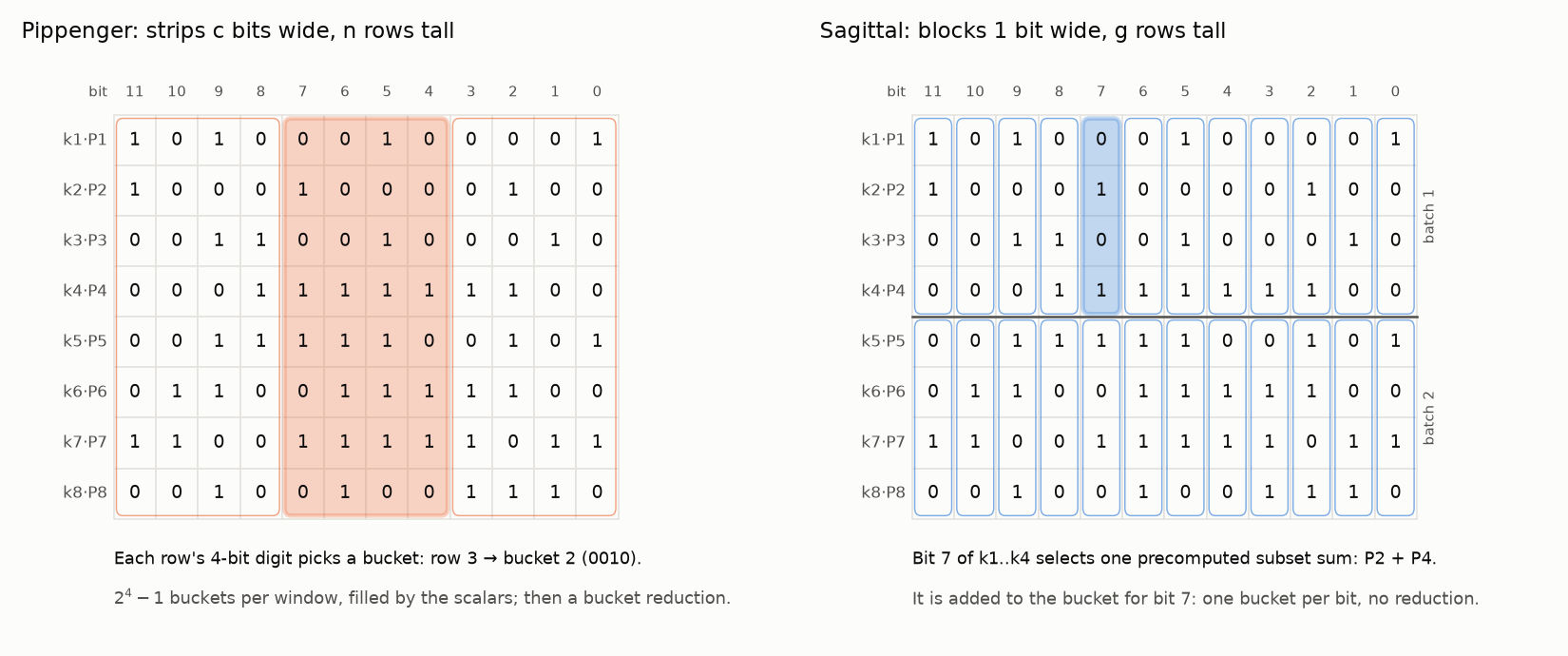
Step 1, once per proving key: build the tables
Each batch of g points gets its own table holding every combination (not permutation: P1 + P2 = P2 + P1) of its points: 2g − 1 entries, each built with one addition from two entries built earlier. Here, 8 points in batches of g = 4 need 2 tables:
Step 2, every proof: look up and add
For each batch and each bit, the g scalar bits form a pattern that picks one table entry, added to the bucket for that bit. There is one bucket per scalar bit. The bit patterns match the table above: 0101 is P2 + P4 in both.
Finally the b buckets (b = 253 scalar bits) are combined with Horner’s rule: start from the top bucket and repeat result = 2·result + bucket[i] down to bit 0, the same doubling chain as double-and-add with bucket i in place of P. That is b − 1 doublings and b − 1 additions in total, about 500 operations whatever n is. There is no bucket reduction, every bucket gets exactly one lookup per batch, and every addition is the cheap mixed kind.
Relation to Straus's method. Straus's method (also called Shamir's trick) computes k1·P1 + … + kg·Pg for a handful of points by precomputing all 2g subset sums, then running one double-and-add over all g scalars together. One Sagittal batch is exactly that. What Sagittal adds:
- every batch runs at once, with one bucket per bit, so the doublings are done only once for all n points instead of once per batch;
- the tables are built offline, once per fixed proving key;
- every bucket's work is fixed before any scalar is read.
Cost formulas and measured counts for every batch size g: docs/4-sagittal.md.
5. Why Sagittal suits GPUs
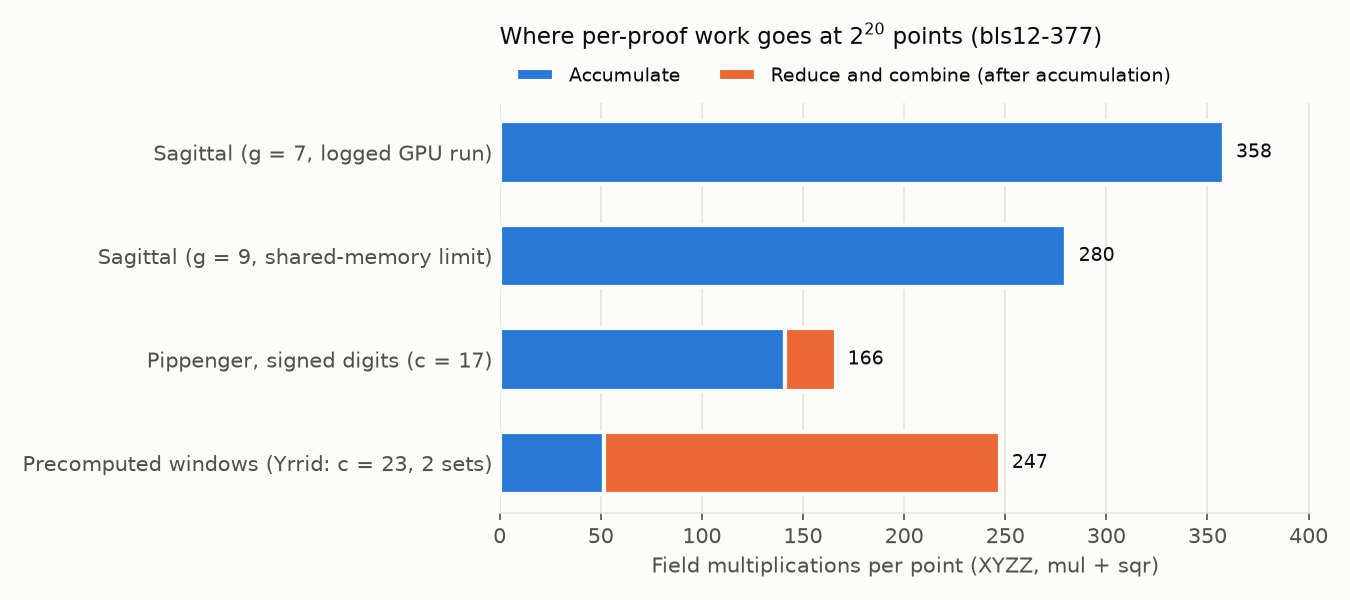
At 220 points Sagittal does more curve operations than a tuned Pippenger. It still ran faster on GPUs in 2023, because of the shape of its work:
- Thread = bit, block = batch. Every thread does one lookup and one addition per batch, so warps don't diverge.
- Tables in shared memory. A batch's 2g entries of 96 bytes fit in 48 KB for g ≤ 9.
- A fixed order. The fastest kernel spreads blocks over 256 copies of the buckets by block number, not by the data, and the 253 final buckets are combined on the CPU.
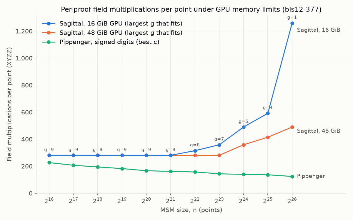
The catch is memory. Tables hold (2g − 1)/g points per input point, so large MSMs force small g. On a 16 GiB V100 the largest g that fits is 8 at 222 and 5 at 224, exactly what the 2023 runs used.
How the kernel maps batches to thread blocks and bits to threads, and why g stays at 9 or below: docs/5-gpu.md.
6. Results
| At 220, per point | Curve operations | Field multiplications |
|---|---|---|
| Sagittal (g = 7) | 35.8 | 358 |
| Precomputed windows (Yrrid config) | 19.1 | 247 |
| Pippenger, signed digits (c = 17) | 15.9 | 166 |
The Yrrid configuration row models the parameters of Yrrid's winning ZPrize entry (c = 23, signed digits, 2 bucket sets), not their code.
Against the Yrrid configuration on the same A10G, Sagittal does 1.87× more curve operations and 1.45× more field multiplications, but was only 1.33× slower (64 vs 48 ms). Field cost explains most of the gap; the shape of the work explains the rest.
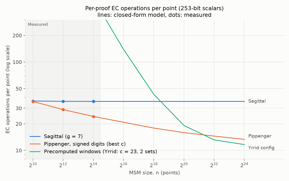
Precompute is cheap. Sagittal's tables cost 385 field multiplications per point to build, about 5× less than the Yrrid configuration's shifted points (2,110). For a single proof, Sagittal costs 743 per point against 2,357; the Yrrid configuration pulls ahead only above 16 proofs per proving key.
Field-cost weighting, precompute and memory in full: docs/6-results.md.
7. How the numbers are made
The repository is a Python reference implementation that counts every operation. Algorithms only call group operations inside named phases, and the group counts them, so the counts always describe the code that ran. They run on BN254, BLS12-377 and a 64-bit Goldilocks test curve (in Jacobian or XYZZ coordinates, with field operations counted too), and on a fast counting group with the same structure. A closed-form model, tested against measured counts within 2%, extends the comparison to 224 points.
The animations above use small examples (8 points, 4–8-bit scalars) so every step fits on
screen. Every number on this page comes from benchmarks/results/ or the 2023 GPU
logs, and the methodology
page lists what they don't cover.
Terms and references
- Field, field element, field multiplication
- The numbers 0 to p − 1, where adding, subtracting, multiplying and dividing all wrap around modulo the prime p. A field element is one such number; a field multiplication multiplies two of them mod p. Curve coordinates are field elements.
- Identity point O, and −P
- The curve's "zero": P + O = P. The negative of P = (x, y) is −P = (x, −y), and P + (−P) = O.
- Circuit, proving key
- A circuit is the computation being proved, written as arithmetic constraints. The proving key is the fixed set of curve points (from a one-time setup) that every proof of that circuit uses. Those points are the Pi of the MSM.
- Affine, Jacobian, XYZZ
- Ways to store a point. Affine is plain (x, y). Jacobian is (X, Y, Z) with x = X/Z², y = Y/Z³. XYZZ is (X, Y, ZZ, ZZZ) with x = X/ZZ, y = Y/ZZZ. The last two avoid division until the end.
- Kernel, thread block, warp, atomic add
- A kernel is a program that runs on the GPU. Its threads are grouped into blocks (up to 1,024 threads sharing fast on-chip memory) and warps (32 threads running one instruction together). An atomic add is a hardware instruction that lets many threads add to the same number without losing updates; it works on single machine numbers, not on curve points.
- n, b, c, g
- n is the number of points (and scalars) in the MSM. b is the number of scalar bits (253 for BLS12-377). c is Pippenger's window width in bits. g is Sagittal's batch size: points per precomputed table.
- Bucket, table entry
- A bucket is a running sum of points. In Pippenger there is one per possible digit value per window; in Sagittal, one per scalar bit. A table entry is one precomputed subset sum of a batch's points.
- Signed digits
- Pippenger window digits from −(2c−1 − 1) to 2c−1 instead of 0 to 2c − 1. A negative digit adds −P, which is nearly free (flipping the sign of y is one field subtraction), so each window needs half as many buckets: 2c−1 instead of 2c.
- Straus's method, Shamir's trick
- Two names for computing k1·P1 + … + kg·Pg by precomputing all 2g subset sums and running one double-and-add over all g scalars together. Straus gave it as the solution to Problem 5125 (Bellman and Straus, American Mathematical Monthly, 1964); the same idea appears in ElGamal's 1985 signature paper. Textbook treatment: Handbook of Applied Cryptography, §14.6.
- Yrrid configuration
- This project's model of the parameters Yrrid used in its winning ZPrize 2022 entry: window c = 23, signed digits, and shifted point copies that fold all windows into 2 bucket sets. It is a model of their algorithm's operation counts, not their code.
- ZPrize
- A 2022 competition to accelerate zero-knowledge proving. Its GPU MSM track (BLS12-377, batches of 226 points) was led by Yrrid and MatterLabs, whose entries were later combined into one (challenge, results, entries).
- BLS12-377, BN254, Goldilocks
- BLS12-377 and BN254 are curves widely used in zero-knowledge proofs (377- and 254-bit fields; 253- and 254-bit scalars). Goldilocks is the prime 264 − 232 + 1, popular because its numbers fit in a 64-bit word (used by Plonky2); this project uses a small test curve over it. BN254 is the curve behind Ethereum's pairing precompiles (EIP-197).
- V100, A10G, Ampere, sppark
- The V100 (2017, Volta generation, 16 GB) and A10G (Ampere generation, 24 GB) are NVIDIA GPUs. Ampere is the 2020 generation; Yrrid's code requires it. sppark is Supranational's open-source GPU library for MSMs and field arithmetic (GitHub); Sindri's kernel used its field and point types.